
Here, an element of the output set is the square of an element from the input set.
Graphically
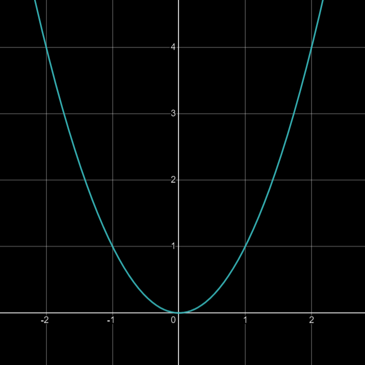
Functions are the fundamental part of the calculus in mathematics.
The functions are the special types of relations.
A function is a mapping between an input set and an output set.
The special condition of a function is that an element of the input set is related to exactly one element of the output set.
Here, an element of the output set is the square of an element from the input set.
(Values that we can take)
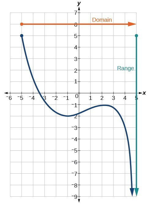
Domain: $[−5,∞)$
Range: $(−∞,5]$
a, b = 3, 4

print("ADDITION OF TWO NUMBERS:")
print(a+b)
ADDITION OF TWO NUMBERS:
7
print("SUBTRACTION OF TWO NUMBERS:")
print(a-b)
ADDITION OF TWO NUMBERS:
-1
print("MULTIPLICATION OF TWO NUMBERS:")
print(a*b)
MULTIPLICATION OF TWO NUMBERS:
-1
print("TRUE DIVISION OF TWO NUMBERS:")
print(a/b)
TRUE DIVISION OF TWO NUMBERS:
0.75
print("FLOOR DIVISION OF TWO NUMBERS:")
print(a//b)
FLOOR DIVISION OF TWO NUMBERS:
0
print("REMAINDER OF TWO NUMBERS:")
print(a%b)
REMAINDER OF TWO NUMBERS:
3
print("POWER OF TWO NUMBERS:")
print(a**b)
POWER OF TWO NUMBERS:
81
a,b = 5, 3

print("Check a is greater than b")
print(a > b)
Check a is greater than b
True
print("Check a is greater than or equal to b")
print(a >= b)
Check a is greater than or equal to b
True
print("Check a is equal to b")
print(a == b)
Check a is equal to b
False
print("Check a is not equal to b")
print( a != b)
Check a is not equal to b
True
print("Check a is less than b")
print(a < b)
Check a is less than b
False
print("Check a is less than or equal to b")
print(a <= b)
Check a is less than or equal to b
False
Math module provides functions to deal with both basic operations such as addition(+), subtraction(-), multiplication(*), division(/) and advance operations like trigonometric, logarithmic, exponential functions.
import math

## constants
print("Euler's Number:", end = " ")
print(math.e)  # euler's number

print("PI:", end = " ")
print(math.pi)  # pi

print("Tau (Ratio of Circumference to the radius of a circle):", end = " ")
print(math.tau) # tau

print("Infinity (never ending):", end = " ")
print(math.inf, end = " ")   # positive infinity
print(-math.inf)  # negative infinity

print("NaN (Not a Number):", end = " " )
print(math.nan) # floating point Not a Number value
Euler's Number: 2.718281828459045
PI: 3.141592653589793
Tau (Ratio of Circumference to the radius of a circle): 6.283185307179586
Infinity (never ending): inf -inf
NaN (Not a Number): nan
import math

a = 2.3
b = -1.3
c = 3

print ("The ceil of 2.3 is : ", end="")
print(math.ceil(a))

print ("The ceil of -1.3 is : ", end="")
print(math.ceil(b))

print ("The ceil of 3 is : ", end="")
print(math.ceil(c))
The ceil of 2.3 is : 3
The ceil of -1.3 is : -1
The ceil of 3 is : 3
It is equivalent to the Least integer function (LIF) in mathematics.
import math

a = 2.3
b = -1.3
c = 3

print ("The floor of 2.3 is : ", end="")
print(math.floor(a))

print ("The floor of -1.3 is : ", end="")
print(math.floor(b))

print ("The floor of 3 is : ", end="")
print(math.floor(c))
The floor of 2.3 is : 2
The floor of -1.3 is : -2
The floor of 3 is : 3
It is equivalent to Greatest integer function (GIF) in mathematics.

import math

a = -10
b = 10

# absolute value or modulus function
print ("The absolute value of -10 is : ", end="")
print (math.fabs(a))

print ("The absolute value of 10 is : ", end="")
print (math.fabs(b))
The absolute value of -10 is : 10.0
The absolute value of 10 is : 10.0

import math

a = 4
b = -3
c = 0.00

# exp() values
print ("The exp() value of 4 is : ", end="")
print (math.exp(a))

print ("The exp() value of -3 is : ", end="")
print (math.exp(b))

print ("The exp() value of 0.00 is : ", end="")
print (math.exp(c))
The exp() value of 4 is : 54.598150033144236
The exp() value of -3 is : 0.049787068367863944
The exp() value of 0.00 is : 1.0
import math

# log of 2,3
print ("The value of log 2 with base 3 is : ", end="")
print (math.log(2,3))

# returning the log2 of 16
print ("The value of log2 of 16 is : ", end="")
print (math.log2(16))

# returning the log10 of 10000
print ("The value of log10 of 10000 is : ", end="")
print (math.log10(10000))
The value of log 2 with base 3 is : 0.6309297535714574
The value of log2 of 16 is : 4.0
The value of log10 of 10000 is : 4.0
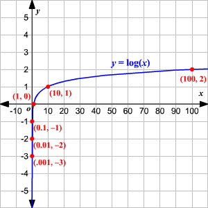
The function $\large y=log_{b}x$ is the inverse function of the exponential function $\large y=b^x$
When no base is written, assume that the log is base 10
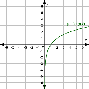
Graph of $log_{2}x$
import math

# print the square root of 0
print ("The square root of 0 is : ", end="")
print(math.sqrt(0))

# print the square root of 4
print ("The square root of 4 is : ", end="")
print(math.sqrt(4))

# print the square root of 3.5
print ("The square root of 3.5 is : ", end="")
print(math.sqrt(3.5))
The square root of 0 is : 0.0
The square root of 4 is : 2.0
The square root of 3.5 is : 1.8708286933869707
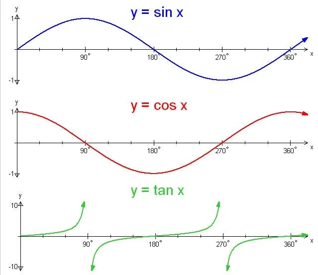
import math

a = math.pi/6

# returning the value of sine of pi/6
print ("The value of sine of pi/6 is : ", end="")
print (math.sin(a))  # value passed must be radians

# returning the value of cosine of pi/6
print ("The value of cosine of pi/6 is : ", end="")
print (math.cos(a))

# returning the value of tangent of pi/6
print ("The value of tangent of pi/6 is : ", end="")
print (math.tan(a))
The value of sine of pi/6 is : 0.49999999999999994
The value of cosine of pi/6 is : 0.8660254037844387
The value of tangent of pi/6 is : 0.5773502691896257
import math

a = math.pi/6
b = 30

# returning the converted value from radians to degrees
print ("The converted value from radians to degrees is : ", end="")
print (math.degrees(a))

# returning the converted value from degrees to radians
print ("The converted value from degrees to radians is : ", end="")
print (math.radians(b))
The converted value from radians to degrees is : 29.999999999999996
The converted value from degrees to radians is : 0.5235987755982988

import math

# initializing argument
gamma_var = 5

# Printing the gamma value.
print ("The gamma value of the given argument is : " + str(math.gamma(gamma_var)))
The gamma value of the given argument is : 24.0
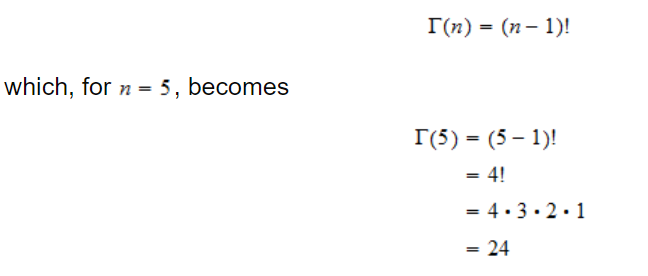
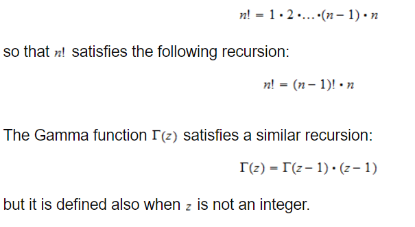
The (complete) gamma function $ \Gamma(n)$ is defined to be an extension of the factorial to complex and real number arguments.
It is often used in probability and statistics, as it shows up in the normalizing constants of important probability distributions such as the Chi-square and the Gamma.

One drawback of all these functions is that they’re not suitable for working with symbolic expressions.
If we want to manipulate a mathematical expression involving symbols, we have to start using the equivalent functions defined by SymPy.
SymPy is a Python library for symbolic mathematics
!pip install sympy --user
Requirement already satisfied: sympy in c:\python311\lib\site-packages (1.12)
Requirement already satisfied: mpmath>=0.19 in c:\python311\lib\site-packages (from sympy) (1.3.0)
import sympy

sympy.sin(math.pi/2)
from sympy import Symbol

theta = Symbol('theta')

# using math
print(math.sin(theta) + math.sin(theta))
---------------------------------------------------------------------------
TypeError                                 Traceback (most recent call last)
Cell In[59], line 6
      3 theta = Symbol('theta')
      5 # using math
----> 6 print(math.sin(theta) + math.sin(theta))

File C:\Python311\Lib\site-packages\sympy\core\expr.py:351, in Expr.__float__(self)
    349 if result.is_number and result.as_real_imag()[1]:
    350     raise TypeError("Cannot convert complex to float")
--> 351 raise TypeError("Cannot convert expression to float")

TypeError: Cannot convert expression to float
# using sympy
print(sympy.sin(theta) + sympy.sin(theta))
2*sin(theta)
from sympy import Symbol

x = Symbol('x')
y = Symbol('y')

z = (x + y) + (x-y)
print("Value of z is: ", z)
Value of z is: 2*x
from sympy import sin, solve, Symbol
u = Symbol('u')
t = Symbol('t')
g = Symbol('g')

theta = Symbol('theta')

solve(u*sin(theta)-g*t, t)
[u*sin(theta)/g]
from sympy import Symbol

x = Symbol('x')

if (x + 5) > 0:
    print("Do something")
else:
    print("Do something else")
---------------------------------------------------------------------------
TypeError                                 Traceback (most recent call last)
Cell In[64], line 5
      1 from sympy import Symbol
      3 x = Symbol('x')
----> 5 if (x + 5) > 0:
      6     print("Do something")
      7 else:

File C:\Python311\Lib\site-packages\sympy\core\relational.py:510, in Relational.__bool__(self)
    509 def __bool__(self):
--> 510     raise TypeError("cannot determine truth value of Relational")

TypeError: cannot determine truth value of Relational
Error thrown because SymPy doesn't know anything about the sign if x, it can't deduce whether x+5 is greather than 0, so it displays an error.
But basic math tells us that if x is positive, x + 5 will always be positive, and if x is negative, it will be positive only in certain cases.
So if we create a Symbol object specifying positive=True, we tell SymPy to assume only positive values.
Now it knows for sure that x + 5 is definitely greater than 0
from sympy import Symbol

x = Symbol('x', positive=True)

if (x + 5) > 0:
    print("Do something")
else:
    print("Do something else")
Do something
If we’d instead specified negative=True, we could get the same error as in the first case.
Just as we can declare a symbol as positive and negative, it’s also possible to specify it as real, integer, complex, imaginary, and so on.
These declarations are referred to as assumptions in SymPy.
A common task in calculus is finding the limiting value (or simply the limit) of the function, when the variable’s value is assumed to approach a certain value.
Consider a function $\Large f(x) = \frac{1}{x}$

As the value of x increases, the value of f(x) approaches 0. Using the limit notation, we'd write this as:

from sympy import Limit, Symbol, S

x = Symbol('x')

Limit(1/x, x, S.Infinity) # unevaluated object
oo denotes positive infinity and the dir='-' symbol specifying that we are approaching the limit from the negative side.
## to find the value of the limit
## use doit() method

l = Limit(1/x, x, S.Infinity)
l.doit()
By default, the limit is found from a positive direction, unless the value at which the limit is to be calculated is positive or negative infinity
Limit(1/x, x, 0, dir='-')
Limit(1/x, x, 0, dir='-').doit()
Limit(1/x, x, 0, dir='+')
Limit(1/x, x, 0, dir='+').doit()
The indeterminate form is a Mathematical expression that means that we cannot be able to determine the original value even after the substitution of the limits.
Indeterminate forms are:
The Limit class also handles functions with limits of indeterminate forms automatically
from sympy import Symbol, sin

Limit(sin(x)/x, x, 0)  # 0/0 form
Limit(sin(x)/x, x, 0).doit()
You have very likely used L’Hospital’s rule to find such limits, but as we see here, the Limit class takes care of this for us.
Futher Reading: https://tutorial.math.lamar.edu/classes/calci/lhospitalsrule.aspx
$\large 1. \lim_{x \to 2} (8 - 3x + 12x^2)$
$\large 2. \lim_{t \to -3} \frac{6 + 4t}{t^2 + 1}$
$\large 3. \lim_{x \to -5} \frac{x^2 - 25}{x^2 + 2x - 15}$
$\large 4. \lim_{z \to -4} \frac{\sqrt z - 2}{z - 4}$
$\large 5. \lim_{t \to -1} \frac{t + 1}{|t+1|}$
For more questions to practice: https://tutorial.math.lamar.edu/problems/calci/computinglimits.aspx
For Latex Guide: https://www.math-linux.com/latex-26/faq/latex-faq/article/latex-derivatives-limits-sums-products-and-integrals
# Q1
from sympy import Limit, Symbol, S

x = Symbol('x')
Limit((8-3*x+12*x**2), x, 2).doit()
# Q2
from sympy import Limit, Symbol, S

t = Symbol('t')
Limit((6+4*t)/(t**2 + 1), t, -3).doit()
# Q3
from sympy import Limit, Symbol, S

x = Symbol('x')
Limit((x**2 - 25)/(x**2 + 2*x - 15), x, -5).doit()
# Q4
from sympy import Limit, Symbol, S

z = Symbol('z')
Limit((z**(0.5) - 2)/(z - 4), z, 4).doit()
# Q5
from sympy import Limit, Symbol, S

t = Symbol('t')

# left hand limit
LHL = Limit((t+1)/(abs(t+1)), t, -1, dir = '-').doit()

# right hand limit
RHL = Limit((t+1)/(abs(t+1)), t, -1, dir = '+').doit()

if LHL == RHL:
    print("Limit exists and value is: ", LHL)
else:
    print("Left Hand Limit is: ", LHL)
    print("Right Hand Limit is: ", RHL)
    print("Since LHL not equal to RHL")
    print("Limits does not exists")
Left Hand Limit is:  -1
Right Hand Limit is:  1
Since LHL not equal to RHL
Limits does not exists
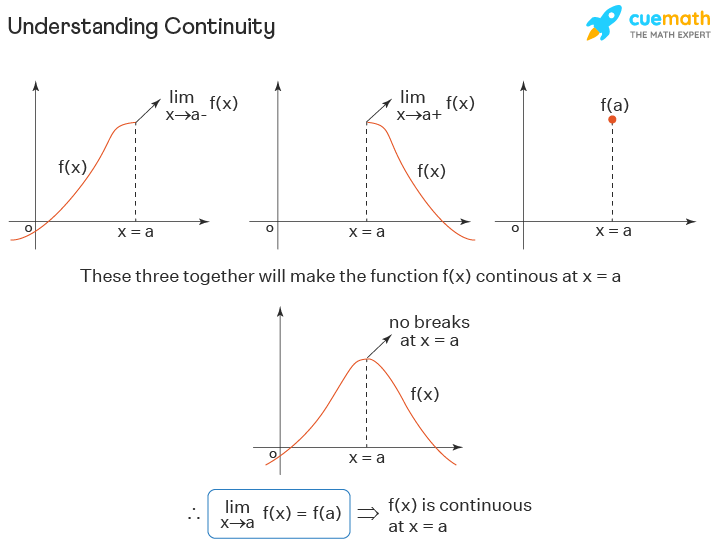
The term 'continuity' is derived from the word continuous, which means an endless or unbroken path.
A real function $\large f(x)$ can be considered as continuous at a point say, $\large x = a$, if the function $\large f(x)$ is approaching to $a$ is $\large f(a)$

Further


# Check the continuity of the function at x = 0
from sympy import Limit, Symbol, S

x = Symbol('x')
f = 5*x - 3
c = 0

# AT x = 0
v = f.evalf(subs = {x: 0})

# left hand limit
LHL = Limit(f, x, 0, dir = '-').doit()

# Right hand limit
RHL = Limit(f, x, 0, dir = '+').doit()

if LHL == RHL == v:
    print("Given function is continuous at x = ", c)
elif LHL != RHL:
    print("Given function is discontinuous at x = ", c)
    print("Type of Discontinuity is: Jump Discontinuity")
elif LHL == RHL:
    print("Given function is discontinuous at x = ", c)
    print("Type of Discontinuity is: Removable Discontinuity")
elif (RHL == math.inf) and (LHL == -math.inf):
    print("Given function is discontinuous at x = ", c)
    print("Type of Discontinuity is: Infinite Discontinuity")
Given function is continuous at x = 0
# Check the continuity of the function at x = 2
from sympy import Limit, Symbol, S

x = Symbol('x')
f = 1/(x-2)
c = 2

# AT x = c
v = f.evalf(subs = {x: c})

# left hand limit
LHL = Limit(f, x, c, dir = '-').doit()

# Right hand limit
RHL = Limit(f, x, c, dir = '+').doit()

if LHL == RHL == v:
    print("Given function is continuous at x = ", c)

elif (RHL == math.inf) and (LHL == -math.inf):
    print("Given function is discontinuous at x = ", c)
    print("Type of Discontinuity is: Infinite Discontinuity")

elif LHL == RHL:
    print("Given function is discontinuous at x = ", c)
    print("Type of Discontinuity is: Removable Discontinuity")

elif LHL != RHL:
    print("Given function is discontinuous at x = ", c)
    print("Type of Discontinuity is: Jump Discontinuity")
Given function is discontinuous at x =  2
Type of Discontinuity is: Infinite Discontinuity
$\large 1. f(x) = (8 - 3x + 12x^2)$ at x = 3
$\large 2. f(x) = \frac{6 + 4t}{t^2 + 1}$ at t = -1
$\large 3. f(x) = \frac{x^2 - 25}{x^2 + 2x - 15}$ at x = 3 and -5
$\large 4. f(x) = \frac{\sqrt z - 2}{z - 4}$ at z = 3
$\large 5. f(x) = \frac{t + 1}{|t+1|}$ at t = -1
Say you have deposited Rs. 1000 in a bank. This deposit is the principal, which pays you interest -- in this case, interest of 100 % that compounds n times yearly for 1 year.
The amount you will get at the end of 1 year is given by
The prominent mathematician James Bernoulli discovered that as the value of n increases, the term $(1 + 1/n)^n$ approaches the value of $e$ — the constant that we can verify by finding the limit of the function:
# lets find out using python
from sympy import Limit, Symbol, S

n = Symbol('n')
l = Limit((1+1/n)**n, n, S.Infinity)
l
l.doit()
For any
principal amount p,
any rate r, and
any number of years t,
the compound interest is calculated using the formula:
from sympy import Symbol, Limit, S

p = Symbol('p', positive = True)
r = Symbol('r', positive = True)
t = Symbol('t', positive = True)

l = Limit(p*(1+r/n)**(n*t), n, S.Infinity)
l
l.doit()
Consider a car moving along a road. It accelerates uniformly such that the distance traveled, S, is given by the function
$S(t) = 5t^2 + 2t + 8$
In this function, the independent variable is t, which represents the time elapsed since the car started moving
If we measure the distance traveled in time $t_1$ and time $t_2$ such that $t_2$ > $t_1$, then we can calculate the distance moved by the car in 1 unit of time using the expression
This is also referred to as the average rate of change of the function $S(t)$ with respect to the variable t, or in other words, the average speed.
If we write the $\large t_{2}$ as $\large t_{1} + \delta_{t}$ -- where $\delta_{t}$ is the difference between $t_{2}$ and $t_{1}$ in units of time -- we can rewrite the expression for the average speed as
Now, if we further assume $\delta_{t}$ to be really small, such that it approached 0, we can use limit notation to write this as
## let's evaluate the above limit

from sympy import Symbol, Limit

t = Symbol('t')
St = 5*t**2 + 2*t + 8

t1 = Symbol('t1')
delta_t = Symbol('delta_t')

St1 = St.subs({t: t1})
St1_delta = St.subs({t: t1 + delta_t})

l = Limit((St1_delta - St1)/ delta_t, delta_t, 0)
l
l.doit()
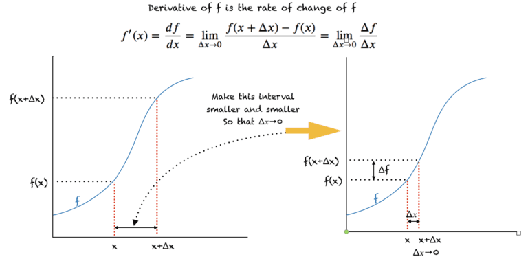
This limit we calculated here is referred to as the derivative of a function, and we can calculate it directly using SymPy's Derivative class.
In very simple words, the derivative of a function $f(x)$ represents its rate of change and is denoted by either $f'(x)$ or $\frac{df}{dx}$.
Let’s first look at its definition and a pictorial illustration of the derivative.
from sympy import Symbol, Derivative

t = Symbol('t')
St = 5*t**2 + 2*t + 8
d = Derivative(St, t)
d
d.doit()
d.doit().subs({t:t1}) # derivative at t = t1
d.doit().subs({t:1}) # derivative at t = 1
$\large f(x) = (x^5 + x^3 + x)*(x^4 + x)$
from sympy import Derivative, Symbol

x = Symbol('x')
f = (x**5 + x**3 + x)*(x**4 + x)
Derivative(f,x).doit()
"""
DERIVATIVE CALCULATOR
"""

from sympy import Symbol, Derivative, sympify, pprint
from sympy.core.sympify import SympifyError

def derivative(f, var):
    var = Symbol(var)
    d = Derivative(f, var).doit()
    pprint(d)

if __name__ == '__main__':
    f = input('Enter a function: ')
    var = input('Enter the variable to differentiate with respect to: ')
    try:
        f = sympify(f) # convert the input function into a SymPy object
    except SympfiyError:
        print("invalid input")
    else:
        derivative(f, var)
Enter a function: 2*x**2 + y**2
Enter the variable to differentiate with respect to: x
4⋅x
A Partial Derivative is a derivative where we hold some variables constant.
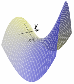
Example: A function for a surface that depends on two variables x and y.
When we find the slope in the x direction (while keeping y fixed) we have found a partial derivative.
Or we can find the slope in the y direction (while keeping x fixed).
from sympy import Derivative, Symbol

x = Symbol('x')
y = Symbol('y')
f = 2*(x**2)*y + x*y**2
Derivative(f,x).doit()
from sympy import Derivative, Symbol

x = Symbol('x')
y = Symbol('y')
f = 2*(x**2)*y + x*y**2
Derivative(f,y).doit()
$\large 1. f(x,y) = x^4 + 6\sqrt y - 10 $
$\large 2. f(x,y,z) = x^2y - 10x^2z^3 + 43x - 7tan(4y)$
$\large 3. f(s,t) = t^7ln(s^2)+ \frac{9}{t^3} - \sqrt(s^4)$
$\large 4. f(x) = cos(\frac{4}{x})e^{x^2y-5y^3}$
Consider the function $\large f(x) = x^5 - 30x^3 + 50x$, defined on the domain [-5,5].

from sympy import Symbol, solve, Derivative

x = Symbol('x')
f = x**5 - 30*x**3 + 50*x
d1 = Derivative(f,x).doit()
d1
critical_points = solve(d1)
critical_points
[-sqrt(9 - sqrt(71)),
 sqrt(9 - sqrt(71)),
 -sqrt(sqrt(71) + 9),
 sqrt(sqrt(71) + 9)]
A = critical_points[2] # global maxima
B = critical_points[0] # local minima
C = critical_points[1] # local maxima
D = critical_points[3] # global minima
## second derivative
d2 = Derivative(f,x,2).doit()
d2
# evaluate second derivative by putting x = B
d2.subs({x:B}).evalf()
# evaluate second derivative by putting x = C
d2.subs({x:C}).evalf()
# evaluate second derivative by putting x = A
d2.subs({x:A}).evalf()
# evaluate second derivative by putting x = D
d2.subs({x:D}).evalf()
Evaluating the second derivative test at the critical points tells us that the points A and C are local maxima and the points B and D are local minima.
The global maximum and minimum of f(x) on the interval [–5, 5] is attained either at a critical point x or at one of the endpoints of the domain (x = –5 and x = 5).
To find the global maximum, we must compute the value of f(x) at the points A, C, –5, and 5. Among these points, the place where f(x) has the largest value must be the global maximum.
x_min = -5
x_max = 5

f.subs({x:A}).evalf()
f.subs({x:C}).evalf()
f.subs({x:x_min}).evalf()
f.subs({x:x_max}).evalf()
To determine the global minimum, we must compute the values of f(x) at the points B, D, –5, and 5:
x_min = -5
x_max = 5

f.subs({x:B}).evalf()
f.subs({x:D}).evalf()
f.subs({x:x_min}).evalf()
f.subs({x:x_max}).evalf()
The indefinite integral, or the antiderivative, of a function f(x) is another function F(x), such that $F′(x) = f(x)$. That is, the integral of a function is another function whose derivative is the original function. Mathematically, it’s written as $F(x) = ∫ f(x)dx$.
The definite integral, on the other hand, is the integral:
where F(b) and F(a) are the values of the anti-derivative of the function at x = b and at x = a, respectively
from sympy import Integral, Symbol

x = Symbol('x')
k = Symbol('k')
I = Integral(k*k, x)
I
I.doit()
I1 = Integral(k*x, (x, 0, 2))
I1
I1.doit()
from sympy import Integral, Symbol

x = Symbol('x')
Integral(x, (x, 2, 4)).doit()
